Examples

SSPROP is distributed with several examples that show how to invoke the program from Matlab. All of the provided examples are taken the first five chapters from G. P. Agrawal’s textbook "Nonlinear Fiber Optics."

We provide one example below, to illustrate the typical usage.

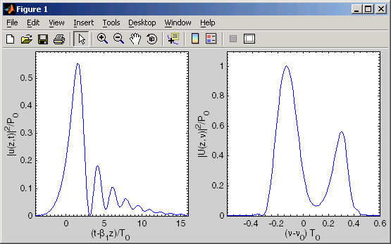
Example: The following m-file demonstrates how to use sspropc (the scalar version) to calculate the pulse shape and spectrum of an unchirped Gaussian pulse after propagating through a fiber with nonlinearity and third-order dispersion. This example replicates Fig. 4.14 from Agrawal’s textbook "Nonlinear Fiber Optics".

T = 100;                     % time window (period)
nt = 2^12;                   % number of points
dt = T/nt;                   % timestep (dt)
t = ((1:nt)'-(nt+1)/2)*dt;   % time vector
w = wspace(T,nt);            % angular frequency vector
vs = fftshift(w/(2*pi));     % shifted for plotting
z = 5;                       % propagation distance
nz = 2000;                   % number of steps
dz = z/nz;                   % step size

betap = [0,0,0,1];           % dispersion polynomial

u0 = gaussian(t,0,2*sqrt(log(2)));  % u0 = exp(-t.^2/2);

u = sspropc(u0,dt,dz,nz,0,betap,1);
U = fftshift(abs(dt*fft(u)/sqrt(2*pi)).^2);

subplot(121);
plot (t,abs(u).^2);
xlim([-4 16]);
xlabel ('(t-\beta_1z)/T_0');
ylabel ('|u(z,t)|^2/P_0');

subplot(122);
plot (vs,U);
xlim([-0.6 0.6]);
xlabel ('(\nu-\nu_0) T_0');
ylabel ('|U(z,\nu)|^2/P_0');

The output of this program is shown below:

Remarks

• In addition to the main computation routine (sspropc), this script uses two other utility routines: gaussian and wspace. These auxiliary utilities are provided as part of SSPROP and are described in the Tools section. The wspace function is used to produce a vector of angular frequencies that correspond to each point in the FFT of the optical signal.
• In this example, we choose nt = 2¹². With the FFTW routines it is no longer necessary to use vector lengths that are powers of two.
• The built-in Matlab command ‘fftshift’ swaps the right and left halves of a vector, which makes it easier to plot.
• Because of the way that the vector w is constructed (see wspace.m), the following commands will produce equivalent plots:
  plot(w,abs(fft(u)).^2);
plot(fftshift(w),fftshift(abs(fft(u)).^2));
  However, the first one will draw the right-half of the spectrum first followed by the left half, connecting the two pieces with a line segment along the horizontal axis.  The second one plots the left half followed by the right as one continuous curve, which looks much better.

• In this example the power spectrum is normalized as follows:
  U = fftshift(abs(dt*fft(u)/sqrt(2*pi)).^2);
  This normalization ensures that the power spectrum will look the same even if you change the period T or the number of points nt.